当前位置：首页 > news >正文

电商网站开发设计方案/整站seo服务

news 2025/6/30 5:51:22

电商网站开发设计方案,整站seo服务,查询个人证件证书查询,网页设计需要什么技术在学习线性回归的时候很多课程都会讲到用梯度下降法求解参数，对于梯度下降算法怎么求出这个解讲的较少，自己实现一遍算法比较有助于理解算法，也能注意到比较细节的东西。具体的数学推导可以参照这一篇博客（梯度下降（Gr…

在学习线性回归的时候很多课程都会讲到用梯度下降法求解参数，对于梯度下降算法怎么求出这个解讲的较少，自己实现一遍算法比较有助于理解算法，也能注意到比较细节的东西。具体的数学推导可以参照这一篇博客（梯度下降（Gradient Descent）小结 - 刘建平Pinard - 博客园）

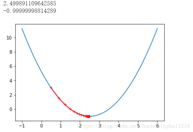
一、首先，我们用一个简单的二元函数用梯度下降法看下算法收敛的过程

也可以改一下eta，看一下步长如果大一点，算法的收敛过程

import numpy as np
import matplotlib.pyplot as pltplot_x = np.linspace(-1,6,140)
plot_y = (plot_x-2.5)**2-1#先算出来当前函数的导数
def dJ(theta):return 2*(theta-2.5)#梯度函数
def J(theta):return (theta-2.5)**2-1#初始化theta=0
#步长eta设置为0.1
eta = 0.1
theta_history = []
theta = 0
epsilon = 1e-8
while True:gredient = dJ(theta)last_theta = thetatheta = theta - eta*gredienttheta_history.append(theta)if(abs(J(theta) - J(last_theta)) < epsilon):breakprint(theta)
print(J(theta))plt.plot(plot_x, J(plot_x))
plt.plot(np.array(theta_history),J(np.array(theta_history)),color='r',marker='+')
plt.show()

出来的结果如下：

二、在线性回归模型中训练算法--批量梯度下降Batch Gradient Descent

首先，构建一个函数

import numpy as np
import matplotlib.pyplot as pltnp.random.seed(666)
x = 2 * np.random.random(size=100)
y = x*3. + 4. + np.random.normal(size=100)#然后改成向量的形式
X = x.reshape(-1,1)plt.scatter(x,y)
plt.show()

然后写实现梯度下降法求解我们构建的这个函数：

def J(theta , X_b , y):try:return sum((y-X_b.dot(theta))**2)/len(X_b)except:return float('inf')#这里使用的是每次求一个参数，然后组合在了一起成了res
def dJ(theta, X_b ,y):res = np.empty(len(theta))res[0] = np.sum(X_b.dot(theta) - y)for i in range(1, len(theta)):res[i] = (X_b.dot(theta) - y).dot(X_b[:,i])return res * 2 / len(X_b)#这里也可以直接用矩阵运算求出所有的参数，效率更高
#return X_b.T.dot(X_b.dot(theta)-y)*2. / len(y)

然后把上面的过程封装成函数形式：

#把整个算法写成函数的形式def gradient_descent(X_b, y ,inital_theta, eta ,n_inters = 1e4, epsilon = 1e-8):theta = initial_thetai_inter = 0while i_inter < n_inters:gradient = dJ(theta, X_b, y)last_theta = thetatheta = theta - eta*gradientif(abs(J(theta,X_b,y) - J(last_theta,X_b,y)) < epsilon):breaki_inter += 1return theta

然后用我们实现的算法求解上面那个函数：

#这里加一列1
X_b = np.hstack([np.ones((len(x),1)), x.reshape(-1,1)])
#初始theta设置为0
initial_theta = np.zeros(X_b.shape[1])
eta = 0.01theta = gradient_descent(X_b, y, initial_theta, eta)
theta

输出结果如下：

array([4.02145786, 3.00706277])

使用梯度下降法时，由于不同维度之间的值大小不一，最好将数据进行归一化，否则容易造成不收敛

三、在线性回归模型中训练算法--随机梯度下降Stochastic Gradient Descent

随机梯度下降法可以训练更少的样本就得到比较好的效果，下面用两段代码比较下。

这个就是之前的批量梯度下降，不过换了一个数据集

import numpy as np
import matplotlib.pyplot as pltm = 100000x = np.random.normal(size = m)
X = x.reshape(-1,1)
y = 4. * x + 3. +np.random.normal(0,3,size = m)def J(theta , X_b , y):try:return sum((y-X_b.dot(theta))**2)/len(X_b)except:return float('inf')def dJ(theta, X_b ,y):return X_b.T.dot(X_b.dot(theta)-y)*2. / len(y) def gradient_descent(X_b, y ,inital_theta, eta ,n_inters = 1e4, epsilon = 1e-8):theta = initial_thetai_inter = 0while i_inter < n_inters:gradient = dJ(theta, X_b, y)last_theta = thetatheta = theta - eta*gradientif(abs(J(theta,X_b,y) - J(last_theta,X_b,y)) < epsilon):breaki_inter += 1return theta

%%time
X_b = np.hstack([np.ones((len(x),1)), X])
initial_theta = np.zeros(X_b.shape[1])
eta = 0.01theta = gradient_descent(X_b, y, initial_theta, eta)
theta

结果如下：

Wall time: 37.2 s

theta：

array([3.00590902, 4.00776602])

下面我们用随机梯度下降：

#这里每次求一行数据的梯度,所以后面不用除以m
def dJ_sgd(theta, X_b_i, y_i):return X_b_i.T.dot(X_b_i.dot(theta) - y_i)* 2. #随机梯度下降法学习率设置t0/(t+t1)这种形式
#由于梯度下降法随机性，设置最后的结果的时候只设置最大迭代次数
def sgd(X_b, y, initial_theta, n_iters):t0 = 5t1 = 50def learning_rate(t):return t0/(t+t1)theta = initial_thetafor cur_iter in range(n_iters):#下面是设置每次随机取一个样本rand_i = np.random.randint(len(X_b))gradient = dJ_sgd(theta, X_b[rand_i], y[rand_i])theta = theta - learning_rate(cur_iter) * gradientreturn theta%%time
X_b = np.hstack([np.ones((len(x),1)), X])
initial_theta = np.zeros(X_b.shape[1])theta = sgd(X_b, y, initial_theta, n_iters=len(X_b)//3)

结果如下：

Wall time: 481 ms

theta:

array([2.93906903, 3.99764075])

对比下两者的运行时间，随机梯度下降法计算量更小，时间也大大减少。

四、小批量梯度下降法-Mini-Batch Gradient Descent

这个完全按照自己理解写下，如果有大牛指点下不胜感激。

小批量梯度下降法主要在于每次训练的数据量不同，随机梯度下降是有一个样本就训练一次，小批量梯度下降是有一批样本训练一次，这里默认参数我给100

#这里每次求一行数据的梯度,所以后面不用除以m
def dJ_sgd(theta, X_b_i, y_i):return X_b_i.T.dot(X_b_i.dot(theta) - y_i)* 2. def sgd(X_b, y, initial_theta, n_iters,n=100):t0 = 5t1 = 50def learning_rate(t):return t0/(t+t1)theta = initial_thetafor cur_iter in range(n_iters):#下面是设置每次随机取一个样本for i in range(n):rand_i = []rand_i_1 = np.random.randint(len(X_b))rand_i.append(rand_i_1)gradient = dJ_sgd(theta, X_b[rand_i], y[rand_i])theta = theta - learning_rate(cur_iter) * gradientreturn theta

然后还是用之前的数据集测试下：

%%time
import numpy as np
X_b = np.hstack([np.ones((len(x),1)), X])
initial_theta = np.zeros(X_b.shape[1])theta = sgd(X_b, y, initial_theta,n=5, n_iters=len(X_b)//3)

结果如下：